Showing posts with label periodic snapshot fact. Show all posts

Monday, September 30, 2013

Adding Min and Max Date Functionality to a Snapshot Fact Table

     When generating periodic snapshots of your data, analysts may want to view that data in ways that may be different than the time frame of capture. For example, you could take snapshots of your company's parts inventory several times a day, once a day, several times a month, once a month, once a quarter, etc. But some analysts may want to report on this data by day, by month, by quarter, by year and by either the state of the inventory by the beginning of the time period or by the end of that period. How do we model this data to allow for this kind of analysis?

     For this example, let's expand upon the company parts and imagine we're dealing with a piece of data that looks like the following and the snapshot schedule is daily:


Figure 1. Source System Inventory Schema


This schema represents the parts inventory quantities, grouped by departments, for a company.  Whenever the data warehouse snapshots the data from this schema a date and time of the snapshot is captured so we can deduce what the inventory state was at that time. 

     In order to fulfill the requirement to report on these snapshots on different time groups, we need a way to categorize this data as such. Now with every data warehouse there will be a date dimension at the level of granularity of the day, in which we could place min/max day/month/quarter/year flags that can help us with this problem. But as you may soon discover, these flags would only pertain to inventory exclusively and if you wanted to use this functionality with other snapshots you would have to add flags specific to that piece of data as well. In addition to this, we may not run this table ETL every day, or if we have an ETL job failure we may miss a day's snapshot. Thus a failure on Sept. 30 means that the Sept 29th snapshot is the maximum one captured for that month. With all of these scenarios, this solution would become untenable very fast. The best way to attack this problem, and provide a re-usable solution, would be to separate these flags out into their own junk dimension. 

     First we need to create this dimension, then determine how we're going to integrate it with the ETL of the snapshot fact table. Our goal is a table that looks like this:


Figure 2. Junk Dimension with Time Flags

-->Create dimension to hold our date categories
CREATE  TABLE  DIM_TIME_FLAG(
    FLAG_KEY        int        NOT NULL,
    MIN_MONTH_FLG   char(1)    NULL,
    MAX_MONTH_FLG   char(1)    NULL,
    MIN_QUARTER_FLG char(1)    NULL,
    MAX_QUARTER_FLG char(1)    NULL,
    MIN_YEAR_FLG    char(1)    NULL,
    MAX_YEAR_FLG    char(1)    NULL,
    CONSTRAINT PK_DIM_TIME_FLAG PRIMARY KEY CLUSTERED (FLAG_KEY)
)

 -->Hold our Y/N enum
DECLARE @enum TABLE
  (
       field char(1)
  )

INSERT INTO @enum(field)values('Y'),('N')

-->Temp table to contain cartesian of Y/N for all fields
DECLARE @final TABLE
 (
        flag_key int identity(1,1),
        field1   char(1),
        field2   char(1),
        field3   char(1),
        field4   char(1),
        field5   char(1),
        field6   char(1)
 )
-->Generate cartesian
INSERT INTO @final
SELECT
        a.field,
        B.field,
        c.field,
        d.field,
        e.field,
        f.field
FROM
        @enum a,
        @enum b,
        @enum c,
        @enum d,
        @enum e,
        @enum f

-->Populate DIM_TIME_FLAG
INSERT INTO DIM_TIME_FLAG
SELECT
       0,
       null,
       null,
       null,
       null,
       null,
       null
UNION
SELECT
       flag_key,
       field1,
       field2,
       field3,
       field4,
       field5,
       field6 
FROM
       @final

-->View Table Rows
SELECT
     FLAG_KEY,
     MIN_MONTH_FLG,
     MAX_MONTH_FLG,
     MIN_QUARTER_FLG,
     MAX_QUARTER_FLG,
     MIN_YEAR_FLG,
     MAX_YEAR_FLG   
FROM
     DIM_TIME_FLAG

We use this table to determine if the record in the snapshot fact is the first/last for the month recorded/quarter recorded/year recorded. The MIN/MAX flags will have values of Y/N and the reporting solution can filter on these flags when trying to report on the various times. For our daily snapshot of parts inventory, we could add this table to a data warehouse schema like this:

Figure 3. Parts Inventory Data Warehouse Schema

     Now, we need to figure out how to get DIM_TIME_FLAG integrated into this schema in our ETL plan. Key thing to keep in mind is that these flags will change as more and more snapshots are taken from the source system. Today's records that have MAX_MONTH_FLG=Y may need to be set to N the following day. After populating the other columns in the table you would have to execute this SQL statement to update the FLAG_KEY:


UPDATE A
SET
       A.FLAG_KEY=Z.FLAG_KEY
FROM
       FCT_PART_INVENTORY A
       INNER JOIN DIM_DAY B ON A.DAY_KEY=B.DAY_KEY
       LEFT JOIN
(
SELECT
       MIN(B.FULL_DATE) AS MIN_MONTH
FROM
       FCT_PART_INVENTORY A
       INNER  JOIN DIM_DAY B ON A.DAY_KEY=B.DAY_KEY
GROUP BY
       B.YEARMO
)MIN_MONTH ON B.FULL_DATE=MIN_MONTH.MIN_MONTH
       LEFT JOIN
(
SELECT
       MAX(B.FULL_DATE) AS MAX_MONTH
FROM
       FCT_PART_INVENTORY A
       INNER  JOIN DIM_DAY B ON A.DAY_KEY=B.DAY_KEY
GROUP BY B.YEARMO
)MAX_MONTH ON B.FULL_DATE=MAX_MONTH.MAX_MONTH
       LEFT JOIN
(
SELECT
       MIN(B.FULL_DATE) AS MIN_QUARTER
FROM
       FCT_PART_INVENTORY A
       INNER  JOIN DIM_DAY B ON A.DAY_KEY=B.DAY_KEY
GROUP BY
       CONVERT(VARCHAR,B.QUARTER)+CONVERT(VARCHAR,B.YEAR)
)MIN_QUARTER ON B.FULL_DATE=MIN_QUARTER.MIN_QUARTER
       LEFT JOIN
(
SELECT
       MAX(B.FULL_DATE) AS MAX_QUARTER
FROM
       FCT_PART_INVENTORY A
       INNER  JOIN DIM_DAY B ON A.DAY_KEY=B.DAY_KEY
GROUP BY
       CONVERT(VARCHAR,B.QUARTER)+CONVERT(VARCHAR,B.YEAR)
)MAX_QUARTER ON B.FULL_DATE=MAX_QUARTER.MAX_QUARTER
       LEFT JOIN
(
SELECT
       MIN(B.FULL_DATE) AS MIN_YEAR
FROM
       FCT_PART_INVENTORY A
       INNER  JOIN DIM_DAY B ON A.DAY_KEY=B.DAY_KEY
GROUP BY
       B.YEAR
)MIN_YEAR ON B.FULL_DATE=MIN_YEAR.MIN_YEAR
LEFT JOIN
(
SELECT
       MAX(B.FULL_DATE) AS MAX_YEAR
FROM
       FCT_PART_INVENTORY A
       INNER  JOIN DIM_DAY B ON A.DAY_KEY=B.DAY_KEY
GROUP BY B.YEAR
)MAX_YEAR ON B.FULL_DATE=MAX_YEAR.MAX_YEAR
LEFT JOIN DIM_TIME_FLAG Z
ON CASE WHEN MIN_MONTH.MIN_MONTH IS NULL THEN 'N' ELSE 'Y' END =Z.MIN_MONTH_FLG
AND CASE WHEN MAX_MONTH.MAX_MONTH IS NULL THEN 'N' ELSE 'Y' END =Z.MAX_MONTH_FLG
AND CASE WHEN MIN_QUARTER.MIN_QUARTER IS NULL THEN 'N' ELSE 'Y' END =Z.MIN_QUARTER_FLG
AND CASE WHEN MAX_QUARTER.MAX_QUARTER IS NULL THEN 'N' ELSE 'Y' END =Z.MAX_QUARTER_FLG
AND CASE WHEN MIN_YEAR.MIN_YEAR IS NULL THEN 'N' ELSE 'Y' END =Z.MIN_YEAR_FLG

AND CASE WHEN MAX_YEAR.MAX_YEAR IS NULL THEN 'N' ELSE 'Y' END =Z.MAX_YEAR_FLG

     With this table now integrated into this schema, we can not only use it at the level of day, but now month, quarter and year all using the same fact. For example, if we wanted to view data across days we can ignore the DIM_TIME_FLAG and simply filter our query across DIM_DAY and report on something that looks like this:

Figure 4. Daily Parts Inventory

     If we need to report on trending across months we could query the exact same snapshot fact, but this time join to DIM_TIME_FLAG where MIN_MONTH_FLG or MAX_MONTH_FLG=Y (depending of if you want to trend over months based on what the inventory looked like at the beginning of the month or end of the month). This would produce a report that would look something like this:

Figure 5. Monthly Parts Inventory

     The same could be done by quarter, as well, using the quarter flags:

Figure 6. Quarterly Parts Inventory

     And finally by year:

Figure 7. Yearly Parts Inventory

     This design can come in very handy, especially when building dashboards and executives want to be able to trend across the different time frames. It also negates the need to create separate snapshot tables that capture this data for each of these time frames(i.e. a snapshot for months, a snapshot for quarters, etc.).

Thursday, May 23, 2013

Using a Pivot to Derive Semi-Additive Measures for a Periodic Snapshot Fact

     Data Modeling can sometimes require more art than science, in that you need to have some kind of creativity when dealing with the "medium" you have been provided. With some source systems you will have complete control over what the data will look like when it gets sent to the data warehouse. Sometimes, you just have to suck it up and deal with what ever format the source system provides you. But with this, comes opportunity. Sometimes not dealing with a third normal form table, and up, can allow you to have everything you need in one neat package. This means dimensions, with attributes, and facts, with measures, that can be derived from 1 piece of data. 

   Take this data representing inventory of some fictional data centers that doesn't even meet the requirements of first normal form due to the repeating groups of data:

Figure 1. Data Center Source Data

Create and Populate:

CREATE TABLE DATA_CENTER_LIST
(
DATA_CENTER_NAME VARCHAR(30),
DATA_CENTER_ADDRESS VARCHAR(30),
DATA_CENTER_CITY VARCHAR(30),
DATA_CENTER_STATE VARCHAR(30),
SERVER_NAME VARCHAR(30),
ATTRIBUTE_TYPE VARCHAR(30),
ATTRIBUTE_VALUE VARCHAR(30)
)
GO

INSERT INTO DATA_CENTER_LIST VALUES
('Data Center 1', '111 Main St', 'Denver', 'CO', 'Server 1', 'OS', 'Windows'),
('Data Center 1', '111 Main St', 'Denver', 'CO', 'Server 1', 'Platform', 'Dell'),
('Data Center 1', '111 Main St', 'Denver', 'CO', 'Server 1', 'Role', 'File Server'),
('Data Center 1', '111 Main St', 'Denver', 'CO', 'Server 2', 'OS', 'Linux'),
('Data Center 1', '111 Main St', 'Denver', 'CO', 'Server 2', 'Platform', 'HP'),
('Data Center 1', '111 Main St', 'Denver', 'CO', 'Server 2', 'Role', 'Web Server'),
('Data Center 1', '111 Main St', 'Denver', 'CO', 'Server 3', 'OS', 'Windows'),
('Data Center 1', '111 Main St', 'Denver', 'CO', 'Server 3', 'Platform', 'HP'),
('Data Center 1', '111 Main St', 'Denver', 'CO', 'Server 3', 'Role', 'SQL Server'),
('Data Center 1', '111 Main St', 'Denver', 'CO', 'Server 4', 'OS', 'Windows'),
('Data Center 1', '111 Main St', 'Denver', 'CO', 'Server 4', 'Platform', 'Dell'),
('Data Center 1', '111 Main St', 'Denver', 'CO', 'Server 4', 'Role', 'File Server'),
('Data Center 1', '111 Main St', 'Denver', 'CO', 'Server 5', 'OS', 'Windows'),
('Data Center 1', '111 Main St', 'Denver', 'CO', 'Server 5', 'Platform', 'HP'),
('Data Center 1', '111 Main St', 'Denver', 'CO', 'Server 5', 'Role', 'File Server'),
('Data Center 2', '10 West Ave', 'Denver', 'CO', 'Server 6', 'OS', 'Windows'),
('Data Center 2', '10 West Ave', 'Denver', 'CO', 'Server 6', 'Platform', 'Dell'),
('Data Center 2', '10 West Ave', 'Denver', 'CO', 'Server 6', 'Role', 'SQL Server'),
('Data Center 2', '10 West Ave', 'Denver', 'CO', 'Server 7', 'OS', 'Linux'),
('Data Center 2', '10 West Ave', 'Denver', 'CO', 'Server 7', 'Platform', 'HP'),
('Data Center 2', '10 West Ave', 'Denver', 'CO', 'Server 7', 'Role', 'Web Server'),
('Data Center 2', '10 West Ave', 'Denver', 'CO', 'Server 8', 'OS', 'Windows'),
('Data Center 2', '10 West Ave', 'Denver', 'CO', 'Server 8', 'Platform', 'HP'),
('Data Center 2', '10 West Ave', 'Denver', 'CO', 'Server 8', 'Role', 'SQL Server'),
('Data Center 2', '10 West Ave', 'Denver', 'CO', 'Server 9', 'OS', 'Windows'),
('Data Center 2', '10 West Ave', 'Denver', 'CO', 'Server 9', 'Platform', 'Dell'),
('Data Center 2', '10 West Ave', 'Denver', 'CO', 'Server 9', 'Role', 'SQL Server'),
('Data Center 2', '10 West Ave', 'Denver', 'CO', 'Server 10', 'OS', 'Linux'),
('Data Center 2', '10 West Ave', 'Denver', 'CO', 'Server 10', 'Platform', 'HP'),
('Data Center 2', '10 West Ave', 'Denver', 'CO', 'Server 10', 'Role', 'Web Server')
GO

This table is ugly, but presents us with a lot of options depending on business requirements. From a first look, we can easily see 2 dimensions we can derive from this data:

Figure 2. Derived Dimensions


We would have to eliminate the repeating groups, and select distinct values for the attributes of both. Once that is done, we can show relationships between the 2 through the use of a fact-less fact like this:

Figure 3. Fact-less Fact
     
     There are more opportunities hidden in this data rather than just deriving relationships between 2 dimensions. Say there was a requirement to snapshot the data center inventory by server attributes, to get a grasp of how inventory is changing periodically. This would be achieved best by making use of a periodic snapshot table. One way of doing this would be to take the attributes of the server and move them to a junk dimension in a schema like this:

Figure 4. Periodic Snapshot Fact Schema with Junk Dimension

     With this solution, we can sum SERVER_COUNT(where server count is the sum of servers with the unique combination of attributes in DIM_SERVER_CATEGORY recorded on the date in DIM_DAY that are tied to a data center in DIM_DATA_CENTER) by data center and server category to determine how many servers per data center have certain attributes. SERVER_COUNT would thus represent a semi-additive measure since we cant aggregate outside of the context we defined for the day.  We can query this schema within certain constraints, like this query used to find the number of servers per data center on 3/15/2013 that had Linux as their OS:

SELECT
       DC.DATA_CENTER_NAME,
       SUM(SERVER_COUNT) AS SERVER_COUNT
 FROM
       FCT_DATA_CENTER_INVENTORY FC
       INNER JOIN DIM_DAY DY ON FC.DAY_KEY=DY.DAY_KEY
       INNER JOIN DIM_DATA_CENTER ON DC.DATA_CENTER_KEY=FC.DATA_CENTER_KEY
       INNER JOIN DIM_SERVER_CATEGORY DS ON FC.SERVER_CATEGORY_KEY=DS.SERVER_CATEGORY_KEY
WHERE
       DY.FULL_DATE='3/15/2013' AND DS.OS='LINUX'
GROUP BY
       DC.DATA_CENTER_NAME

     This should fulfill the business requirement for inventory snapshots. But we can look at this in another way as well. What if this schema doesn't sit well with your report developers. They like that its much easier to deal with than the format of the source system data, but they want it even simpler. They don't like the junk dimension and would much rather see the measures transposed across the fact in a schema like this:

Figure 5. Periodic Snapshot Fact with Transposed Measures
    
     This is a little less flexible than the last schema and only fits a specific requirement. But it is easy to query and takes the need to do the transpose away from the reporting solution. However; it removes the ability to slice and dice across the junk dimension. But if that's what they want, and you've communicated the restrictions to the business, then so be it!

     In order for us to start the ETL process for this periodic snapshot, we would need a separate process to populate the DIM_DATA_CENTER from the same piece of source data before we can populate this fact. This would entail selecting distinct values from the source table (in this example we'll call this DATA_CENTER_LIST) and slapping a surrogate key on the table. This would be from a de-duping mechanism or just a distinct in SQL:

SELECT DISTINCT
       DATA_CENTER_NAME ,
       DATA_CENTER_ADDRESS ,
       DATA_CENTER_CITY ,
       DATA_CENTER_STATE
FROM
       DATA_CENTER_LIST

     With the dimension created and populated we can focus on the ETL for FCT_DATA_CENTER_INVENTORY. There are 2 ways to go about this, from a sourcing perspective, and I'll examine both in the next section here. This first way of going about it is to take advantage of the tools provided by SSIS, primarily the Pivot Transformation. For this our data flow would look similar to this(disregard the Union All Transformation, that's here so we can have a data viewer to view the output, in a normal implementation this would go to a data destination):

Figure 6. Data Flow with Pivot

     In order for us to be able to use the Pivot Transformation as it was designed, we need to prep the data a little to avoid duplicate pivot key errors. To pre-aggregate the data we'll use this query as our OLE DB Source:

SELECT 
         DATA_CENTER_NAME
        ,ATTRIBUTE_VALUE
        ,SUM(1) as TOTAL
FROM  
        DATA_CENTER_LIST
GROUP BY
        DATA_CENTER_NAME
       ,ATTRIBUTE_VALUE

Which will produce this data set:


Figure 7. Pre-Aggregated Data

This will be used as our input for the Pivot Transformation. On the Input Columns Tab we need to select the 3 columns from the source query as an input:

Figure 8. Pivot Input Columns Tab

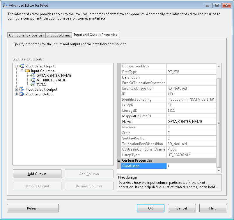
     Next, we need to configure our Input and Output Properties. On the Input and Output Properties Tab we need to first set up our Pivot Default Input properly. For this section we need to be focused primarily on what type of role each input column is going to play in this pivot. These are the different types we have to choose from:

Figure 9. Pivot Usage Options

     Our input column DATA_CENTER_NAME will be assigned a 1 since this is part of the key for this set of data, ATTRIBUTE_VALUE will be assigned a 2 since we want to pivot off of the values in this column and TOTAL will be 3 since these will be our values when the pivot completes. These numbers are entered in PivotUsage under Custom Properties:

Figure 10. Pivot Usage


     With these all configured properly, we move on to the Pivot Default Output node. Here we need to map our input columns to output columns and configure our pivot key column (DATA_CENTER_NAME):

Figure 11. Pivot Default Output

     Here is where we enter all of our measures, these need to both be mapped to an input column and have a PivotKeyValue set. The PivotKeyValue will be the value in ATTRIBUTE_VALUE we want to transpose on. For the NUM_FILE_SERVER column this will be "File Server". Now, this column needs to be mapped to the TOTAL column through SourceColumn. Here you can see that the value is 1963. This is the same as the LineageID of the TOTAL column in the input columns:

Figure 12. TOTAL LineageID

     This needs to be repeated for all of the NUM_* columns in the output, except for PivotKeyValue, enter the unique value for each (i.e. Linux, HP, Dell, Windows...etc). The last thing we need to do for this pivot is configure the DATA_SOURCE_NAME column on the output. For this step we set the SourceColumn to 1911, which is the LineageID for the DATA_SOURCE_NAME input column (see figure 10). With this in place we can run the package and see what the data looks like through a data viewer:

Figure 13. Pivot Transform Output


     As you can see here, all the columns are pivoted on the different values in ATTRIBUTE_VALUE. But this data is still not ready for our fact, we have nulls and repeating DATA_CENTER_NAME values. To finish this we will need to aggregate the values in an Aggregate Transformation and get the current date, of the snapshot, out of a Derived Column Transformation. For the Aggregate Transformation, we need to group by the DATA_CENTER_NAME and sum the NUM_* columns:

Figure 14. Aggregate Transformation Editor

     This will take care of the null values for the NUM_* columns and the repeating values for DATA_CENTER_NAME. Now we just need to get the current date added to the data flow and handle any left over nulls(because there is a 0 value for it in the source data) through the Derived Column Transformation:

Figure 15. Derived Column Transformation Editor

     Lets run the package again and see what our data looks like in the data viewer:

Figure 16. Aggregated Data

     This data is now in the format we need. We can add 2 Lookup Transformations, 1 for  DIM_DATA_CENTER and 1 for DIM_DAY. This will add DATA_CENTER_KEY and DAY_KEY to our data flow, which is the last 2 columns we need to populate FCT_DATA_CENTER_INVENTORY. 

     We now have implemented an ETL strategy for our FCT_DATA_CENTER_INVENTORY using pivot and aggregate. But this is not the only way to do this. We could essentially cut out the "middle man" of the pivot and aggregate transformations by utilizing a pivot statement in conjunction with a cross apply in SQL. This will allow us to pivot our data right in the OLE DB Source:

SELECT
       PVT_OS.DATA_CENTER_NAME,
       SUM(ISNULL([WINDOWS],0)) AS NUM_WINDOWS,
       SUM(ISNULL([LINUX],0))   AS NUM_LINUX,
       SUM(NUM_HP)              AS NUM_HP,
       SUM(NUM_DELL)            AS NUM_DELL,
       SUM(NUM_SQL_SERVER)      AS NUM_SQL_SERVER,
       SUM(NUM_WEB_SERVER)      AS NUM_WEB_SERVER,
       SUM(NUM_FILE_SERVER)     AS NUM_FILE_SERVER
FROM
(
SELECT
       DATA_CENTER_NAME,
       ATTRIBUTE_VALUE,
    1 AS OS_COUNT
FROM
       DATA_CENTER_LIST
WHERE
       ATTRIBUTE_TYPE='OS'

)
p PIVOT ( SUM(OS_COUNT)
                    FOR ATTRIBUTE_VALUE  IN ([WINDOWS],[LINUX])
                  ) AS PVT_OS

CROSS APPLY

            (
             SELECT
              DATA_CENTER_NAME,
              SUM(ISNULL([HP],0)) AS NUM_HP,
              SUM(ISNULL([DELL],0)) AS NUM_DELL
             FROM
                 (
                   SELECT
                     DATA_CENTER_NAME,
                     ATTRIBUTE_VALUE,
                     1 AS PLATFORM_COUNT
                    FROM
                     DATA_CENTER_LIST
                    WHERE
                     ATTRIBUTE_TYPE='PLATFORM'

                  )
                     p PIVOT ( SUM(PLATFORM_COUNT)
                     FOR ATTRIBUTE_VALUE  IN ([HP],[DELL])
             ) AS PVT_PLATFORM
WHERE
 PVT_PLATFORM.DATA_CENTER_NAME=PVT_OS.DATA_CENTER_NAME
GROUP BY 
 DATA_CENTER_NAME

             )PVT_PLATFORM

CROSS APPLY

             (
              SELECT
               DATA_CENTER_NAME,
               SUM(ISNULL([SQL SERVER],0)) AS NUM_SQL_SERVER,
               SUM(ISNULL([WEB SERVER],0)) AS NUM_WEB_SERVER,
               SUM(ISNULL([FILE SERVER],0)) AS NUM_FILE_SERVER
              FROM
                  (
                    SELECT
                     DATA_CENTER_NAME,
                     ATTRIBUTE_VALUE,
                     1 ROLE_COUNT
                    FROM
                     DATA_CENTER_LIST
                    WHERE
                     ATTRIBUTE_TYPE='ROLE'

                   )
         p PIVOT ( SUM(ROLE_COUNT)
         FOR ATTRIBUTE_VALUE  IN ([SQL SERVER],[WEB SERVER], [FILE SERVER])
               ) AS PVT_ROLE
WHERE
 PVT_ROLE.DATA_CENTER_NAME=PVT_OS.DATA_CENTER_NAME 
GROUP BY 
 DATA_CENTER_NAME

             )PVT_ROLE

GROUP BY 
       PVT_OS.DATA_CENTER_NAME

     
     Executing this statement gives you (drum roll):

Figure 17. Pivot SQL Results

The same results we got after we passed the data through the Pivot Transformation, Aggregate Transformation and Derived Column Transformation. So there are options here. But it all depends on your comfort level with using pivot in SQL. The transformations in SSIS do the same thing as the SQL and sometimes using a tool can help demystify some of this data.

     Look at all the things we are able to do with just a little piece of non-normalized data. We were able to derive 3 dimensions,3 facts and 2 ETL strategies. Pretty incredible given the right tool set.