Showing posts with label data modeling. Show all posts

Friday, November 22, 2013

Designing and Populating a Mini-Dimension

     Dealing with master data can be a headache.....a big one. One of these headaches is when large dimensions (millions of rows) contains rapidly changing attributes, or what Kimball refers to as monster dimensions. Now to solve this problem you could go with a traditional SCD type 2, and simply insert a new record every time a change occurs. But due to the rate of change this just doesn't seem tenable. If you had 2 million master data records in your dimension, and even if they only change once a year, that's a million new records in that table every year. Imagine if it was every month, week, day? 

     Luckily, to address this issue we can take advantage of a modeling trick called a mini-dimension. With a mini-dimension, we separate the rapidly changing attributes from the dimension and add them to their own dimension. This eliminates the need to add more records to the dimension every time a change takes place. In this post I'll be describing how to implement a SCD type 4 in your schema, which takes advantage of a mini-dimension.

     For this example, lets use a source system schema such as this:

Figure 1. Source System Schema
     This represents a service transaction on a product, for example's sake it doesn't matter what kind of service, just that a transaction at a point in time involved a customer's product. We have the product being serviced, the customer who owns the product, the employee who serviced the product and when the service took place.  Now, deriving a dimensional schema from this appears rather simple, and would probably look something like this:
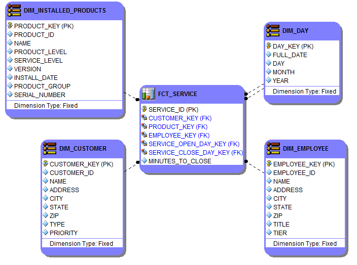
Figure 2. Dimensional Schema

     It's simple and easy to understand, reporting out of this schema should not be a problem. However; what if the version of the product changes very often, impacting the product level and service level attributes, and the number of installed products goes up into the millions? Implementing an SCD type 2 probably wouldn't be a good choice. For this type of situation, were going to pull the rapidly changing attributes out of DIM_INSTALLED_PRODUCTS and put them into their own dimension:

Figure 3. Dimensional Schema with Mini-Dimension

     With the addition of DIM_PRODUCT_VERSION we can see what the product version, product level and service level were at the time of the transaction as well as what they are now (make those attributes SCD type 1 in DIM_INSTALLED_PRODUCTS).

     Now that we have this modeled out we need to figure out how to populate this new dimension and link it to FCT_SERVICE.  Let's generate some sample data, stage it into a persistent staging database (integration layer in your architecture)and then populate the dimension. 

-->Source System Table
CREATE TABLE INSTALLED_PRODUCTS
(
       PRODUCT_ID INT NOT NULL,
       NAME VARCHAR(20),
       PRODUCT_LEVEL INT,
       SERVICE_LEVEL INT,
       VERSION VARCHAR(10),
       INSTALL_DATE DATETIME,
       PRODUCT_GROUP VARCHAR(25),
       SERIAL_NUMBER VARCHAR(10),
       CUSTOMER_ID INT ,
       CONSTRAINT PK_INSTALLED_PRODUCTS PRIMARY KEY(PRODUCT_ID)
)
GO

-->Sample Data
INSERT INTO
       INSTALLED_PRODUCTS
       (PRODUCT_ID,NAME,PRODUCT_LEVEL,SERVICE_LEVEL,VERSION,INSTALL_DATE,PRODUCT_GROUP,SERIAL_NUMBER,CUSTOMER_ID)
VALUES
       (1, 'PRODUCT A', 1, 2, 'V1.1', '09/01/2013', 'HIGH END', '12345GR4', 1),
       (2, 'PRODUCT B', 5, 1, 'V2.1', '11/14/2010', 'LOW END', '7555655YY8', 4),
       (3, 'PRODUCT C', 7, 5, 'V3.5', '02/17/2008', 'HIGH END', '43789HDKH', 8),
       (4, 'PRODUCT D', 2, 5, 'V7.2', '05/22/2012', 'LOW END', '2956DHD55', 9)
GO

When adding this data to a persistent staging database table, let's call it P_STG_INSTALLED_PRODUCTS, it may end up looking something like this:

Figure 4. Data in Persistent Staging
     Here we inserted all the data from the source system, marked the date it was valid from, set the valid to date to some time way out in the future, and generated hash values for each record. Say 10 days later a change happens to PRODUCT A, we compare the hash of the data coming in from staging with the hash existing in persistent staging, determine if they are different and if so insert a new record:

Figure 5. Record Change in Persistent Staging
     When inserting this new record, we need to be sure to update the previous version of this record to have the VALID_TO date set the end of the day right before the change. With some sample data generated, lets populate our mini-dimension. To populate this dimension, were going to treat it just like a junk dimension  by just inserting unique combinations of these attributes and only combinations that exist in the source system table.

SELECT DISTINCT
       PRODUCT_LEVEL,
       SERVICE_LEVEL,
       VERSION
FROM
       P_STG_INSTALLED_PRODUCTS P_STG
WHERE
    NOT EXISTS(
                 SELECT
                        1
                 FROM
                        DIM_PRODUCT_VERSION DPV
                 WHERE
                        P_STG.PRODUCT_LEVEL=DPV.PRODUCT_LEVEL
                        AND P_STG.SERVICE_LEVEL=DPV.SERVICE_LEVEL
                        AND P_STG.VERSION=DPV.VERSION
              )

     This query, along with generating a surrogate key for the dimension, can be used to populate our DIM_PRODUCT_VERSION mini-dimension. Next, we need to figure out how to incorporate this mini-dimension into the loading of the FCT_SERVICE table. Lets create some sample data to work with for this example.

-->Source System Table
CREATE TABLE SERVICE
(
       SERVICE_ID INT NOT NULL,
       SERVICE_OPEN_DATE DATETIME NOT NULL,
       SERVICE_CLOSE_DATE DATETIME,
       PRODUCT_ID INT NOT NULL,
       CUSTOMER_ID INT NOT NULL,
       EMPLOYEE_ID INT NOT NULL,
       CONSTRAINT PK_SERVICE PRIMARY KEY(SERVICE_ID),
       CONSTRAINT FK_SERVICE_PRODUCT_ID  FOREIGN KEY  (PRODUCT_ID)  REFERENCES  INSTALLED_PRODUCTS(PRODUCT_ID),
       CONSTRAINT FK_SERVICE_CUSTOMER_ID FOREIGN KEY  (CUSTOMER_ID) REFERENCES  CUSTOMER(CUSTOMER_ID),
       CONSTRAINT FK_SERVICE_EMPLOYEE_ID FOREIGN KEY  (EMPLOYEE_ID) REFERENCES  EMPLOYEE(EMPLOYEE_ID)
)
GO

-->Sample Data
INSERT INTO
       SERVICE
       (SERVICE_ID,SERVICE_OPEN_DATE,SERVICE_CLOSE_DATE,PRODUCT_ID,CUSTOMER_ID,EMPLOYEE_ID)
VALUES
       (1, '11/25/2013 10:22:33.324','11/25/2013 11:45:22.432', 1, 1, 7),
       (2, '11/26/2013 16:37:21.876','11/27/2013 10:21:54.765', 2, 4, 9),
       (3, '11/28/2013 19:29:48.768','11/28/2013 22:25:12.472', 3, 8, 7),
       (4, '12/05/2013 05:09:12.354','12/05/2013 07:16:08.009', 4, 9, 7),
       (5, '12/11/2013 07:12:32.312','12/12/2013 23:25:14.764', 1, 1, 7)
      
GO

     This data would eventually be inserted into a persistent staging table just like we did for INSTALLED_PRODUCTS, with P_STG_INSTALLED_PRODUCTS, lets call this table P_STG_SERVICE. This will be the primary table we will look at when trying to generate the data for our FCT_SERVICE table. You'll notice that from the data in SERVICE, that there are 2 transactions for PRODUCT_A. One that occurred before the row in INSTALLED_PRODUCTS was updated and one after. So were going to want to join to DIM_PRODUCT_VERSION on values that matched the values in INSTALLED_PRODUCTS at the time of the transaction for that product in SERVICE. This can be achieved, by populating FCT_SERVICE, in a query like this:


SELECT
  P_SRV.SERVICE_ID,
  CUST.CUSTOMER_KEY,
  PROD.PRODUCT_KEY,
  EMP.EMPLOYEE_KEY,
  OPEND.DAY_KEY AS SERVICE_OPEN_DAY_KEY,
  ISNULL(CLOSED.DAY_KEY,0) AS SERVICE_CLOSE_DAY_KEY,
  PVR.PRODUCT_VERSION_KEY,
  CASE WHEN P_SRV.SERVICE_CLOSE_DATE IS NOT NULL
       THEN DATEDIFF(MI,P_SRV.SERVICE_OPEN_DATE, P_SRV.SERVICE_CLOSE_DATE)
       ELSE NULL
       END AS MINUTES_TO_CLOSE
FROM
  P_STG_SERVICE P_SRV
  INNER JOIN DIM_CUSTOMER CUST ON P_SRV.CUSTOMER_ID=CUST.CUSTOMER_ID
  INNER JOIN DIM_INSTALLED_PRODUCTS PROD ON P_SRV.PRODUCT_ID=PROD.PRODUCT_ID
  INNER JOIN DIM_EMPLOYEE EMP ON P_SRV.EMPLOYEE_ID = EMP.EMPLOYEE_ID
  INNER JOIN DIM_DAY OPEND ON TRY_PARSE(P_SRV.SERVICE_OPEN_DATE AS DATE)=OPEND.FULL_DATE
  LEFT  JOIN DIM_DAY CLOSED ON TRY_PARSE(P_SRV.SERVICE_CLOSE_DATE AS DATE)=CLOSED.FULL_DATE
  INNER JOIN P_STG_INSTALLED_PRODUCTS P_PRD ON P_SRV.PRODUCT_ID=P_PRD.PRODUCT_ID AND P_SRV.SERVICE_OPEN_DATE BETWEEN P_PRD.VALID_FROM AND P_PRD.VALID_TO
  INNER JOIN DIM_PRODUCT_VERSION PVR ON PVR.PRODUCT_LEVEL = P_PRD.PRODUCT_LEVEL AND PVR.SERVICE_LEVEL=P_PRD.SERVICE_LEVEL AND PVR.VERSION=P_PRD.VERSION

     With this solution, we'll be able to see what the product's product level, service level and version were at the time of service in DIM_PRODUCT_VERSION as well as seeing what these values currently are today in DIM_INSTALLED_PRODUCTS.

Thursday, August 1, 2013

Implementing an Aging Bucket Dimension in Your Schema

     For any organization that has any kind of service ticketing system, for either internal or external customers, similar questions are usually raised regardless of the service provided. A major concern for these organizations is issue aging. How many tickets are open now, how long have they been open, on average how long do certain issues stay open. If using a dimensional design pattern, modeling this scenario is easy in that we can create a measure in a fact that will show the amount of days between the open and close date of an issue. However; management likes to "bucket" aging in order to categorize and prioritize. In order to accommodate a business requirement such as this, and make it easy for report developers, we can create an aging bucket dimension that will categorize these issues for us. This bucket would contain the ranges specified by the business and may look something like this:


CREATE TABLE DIM_AGING_BUCKET
(
     AGING_BUCKET_KEY INT NOT NULL,
     AGING_BUCKET_DESC NVARCHAR(35),
     BEGIN_DAY_RANGE INT,
     END_DAY_RANGE INT,
     CONSTRAINT PK_DIM_SERVICE_REQUEST_AGING_BUCKET PRIMARY KEY CLUSTERED (AGING_BUCKET_KEY) 
)
GO

INSERT INTO DIM_AGING_BUCKET
VALUES
(0, NULL, NULL, NULL),
(1, '0 DAYS', -1, 0),
(2, '1-3 DAYS',1,3),
(3, '4-5 DAYS', 4,5),
(4, '6-15 DAYS', 6,15),
(5, '16-30 DAYS', 16,30),
(6, '31-60 DAYS', 31,60),
(7, '61-90 DAYS', 61,90),
(8, '91-120 DAYS', 91,120),
(9, '121-180 DAYS', 121,180),
(10,'181-360 DAYS', 181,360),
(11,'OVER 360 DAYS',361,50000)

GO

     For this example were going to use data from an imaginary table that has staged issue ticket data. This data contains the issue identifier (a degenerate dimension), the natural key for the transaction type, the natural key for the employee assigned to the issue, the natural key of the customer associated to the issue, and the open and close dates of the issue. We can represent this with this sample data:


CREATE TABLE STG_TRANSACTION_RECORDS
(
       TRANSACTION_NO INT,
       TRANSACTION_TYPE_ID INT,
       EMPLOYEE_ID INT,
       CUSTOMER_ID INT,
       TRANSACTION_OPEN_DATE DATETIME,
       TRANSACTION_CLOSE_DATE DATETIME
)

INSERT INTO STG_TRANSACTION_RECORDS(TRANSACTION_NO, TRANSACTION_TYPE_ID, EMPLOYEE_ID, CUSTOMER_ID, TRANSACTION_OPEN_DATE, TRANSACTION_CLOSE_DATE)
VALUES
(1, 2, 5, 7, '1/1/2012','1/5/2012'),

(2, 3, 6, 9, '5/1/2012','6/20/2012'),

(3, 8, 22, 61, '12/22/2012','4/1/2013'),

(4, 7, 11, 13, '7/9/2013','7/22/2013'),

(5, 9, 22, 47, '7/23/2013',NULL)

GO

We want to be able to load this data into a star schema that will utilize our bucket dimension. This schema may look something like this:

Figure 1. Star Schema with Bucket Dimension

     Now in order to populate the fact table we would need to join the staging table to the dimensions on the natural keys and retrieve the surrogate keys from these dimensions. The measures (DAYS_OPEN) would simply be a datediff between the open and close dates and (NUMBER_TRANSACTION) will always be a 1 so we can sum on this across the dimensions. This leaves us with one problem, how do we join to DIM_AGING_BUCKET if we have no natural key in either the dimension or the staging table? We in essence are forced to join on a range. This SQL statement will gather up our surrogate keys, calculate our measure and handle the "range join" we need for our bucket dimension:

SELECT
   STG.TRANSACTION_NO,
   CUST.CUSTOMER_KEY,
   AG.AGING_BUCKET_KEY
   AGING_BUCKET_KEY,
   TYP.TRANSACTION_TYPE_KEY,
   EMP.EMPLOYEE_KEY,
   OPEND.DAY_KEY AS OPEN_DAY_KEY,
   ISNULL(CLOSED.DAY_KEY,0) AS CLOSE_DAY_KEY,
   DATEDIFF(DAY, STG.TRANSACTION_OPEN_DATE, CASE WHEN STG.TRANSACTION_CLOSE_DATE IS NULL THEN GETDATE() ELSE STG.TRANSACTION_CLOSE_DATE END)  as DAYS_OPEN,
 AS NUMBER_TRANSACTION

FROM
   STG_TRANSACTION_RECORDS STG
 JOIN DIM_TRANS_TYPE TYP ON STG.TRANSACTION_TYPE_ID=TYP.TRANSACTION_TYPE_ID
 JOIN DIM_EMPLOYEE EMP ON STG.EMPLOYEE_ID=EMP.EMPOYEE_ID
 JOIN DIM_CUSTOMER CUST ON STG.CUSTOMER_ID=CUST.CUSTOMER_ID
 JOIN DIM_DAY OPEND ON STG.TRANSACTION_OPEN_DATE =OPEND.FULL_DATE
 LEFT JOIN DIM_DAY CLOSED ON STG.TRANSACTION_CLOSE_DATE=CLOSED.FULL_DATE
 JOIN DIM_AGING_BUCKET AG ON DATEDIFF(DAY, STG.TRANSACTION_OPEN_DATE, CASE WHEN STG.TRANSACTION_CLOSE_DATE IS NULL THEN GETDATE() ELSE STG.TRANSACTION_CLOSE_DATE END) BETWEEN AG.BEGIN_DAY_RANGE AND AG.END_DAY_RANGE

     As long as your bucket ranges do not overlap, a join based on a range should be fine. Now you can group by the buckets in DIM_AGING_BUCKET while summing on the NUMBER_TRANSACTION field to display the number of issues in the bucket.

Monday, June 17, 2013

Reverse Engineering an Analysis Services Cube using SSIS

     When using the Microsoft BI Stack, cubes are usually seen as the end of the road(kind of). They are usually built on top of facts and dimensions in your data warehouse/data marts. These represent the culmination of all of your team's hard work. The requirements gathering/analysis, ETL/ELT, data warehouse design, reports/analytics and UAT, etc. However; these same end user destinations may, in certain situations, be the only point of exposure to other data systems. If you are tasked with pulling down data into your data warehouse from some other data store's cube then, in essence, their end is your beginning. Luckily SSIS can help with this.

     For this example, we're are going to be modeling data that tracks the complaint to event ratio for a certain range of products over a given time frame. We're going to be using a cube called "Events":

Figure 1. Event Cube

     In order to extract the data we want, we need to focus on measures COMPLAINT QT, EVENT QTY and dimensions ADD DAY and DIM PRODUCT. Now, when looking at cubes we have to remember that they are multidimensional and not 2 dimensional as tables in a database are. So we simply can't use a SQL statement to get the data we need, we'll have to use Multidimensional Expressions (MDX). For this, we're going to need to use 2, one to get the measures(facts) and one for the product(dimension). For the measures we're going to use this MDX statement:

WITH MEMBER [MEASURES].[COMPLAINT RATIO] as '([MEASURES].[COMPLAINT QTY] / [MEASURES].[EVENT COUNT])',FORMAT_STRING='0.00'
MEMBER [MEASURES].[COMPLAINT_QTY] as '[MEASURES].[COMPLAINT QTY] +0'
MEMBER [MEASURES].[EVENT_COUNT] as '[MEASURES].[EVENT COUNT] +0'
MEMBER [MEASURES].[COMPLAINT_RATIO] as '[MEASURES].[COMPLAINT RATIO] +0'

SELECT

{
       [MEASURES].[COMPLAINT_QTY],
       [MEASURES].[EVENT_COUNT],
       [MEASURES].[COMPLAINT_RATIO]
ON COLUMNS,

(
       {
              [DIM PRODUCT].[MODEL].CHILDREN
       },
        
       {
              [ADD DAY].[Hierarchy].[FULL DATE].MEMBERS
       }
 ) ON ROWS
FROM
        EVENTS
WHERE
    (
       [ADD DAY].[YEARMO].[201301] : [ADD DAY].[YEARMO].[201303]
    )

     This statement will return the number of complaints, events and complaint to event ratio(non-additive) by product model for first quarter 2013. We want all the product model children in this result set and by adding this we make sure we don't return a summation set. We also want all of the full date members, which will return all the dates at that level of the hierarchy.

Figure 2. Measures MDX Result Sample
     This takes care of our measures. Now we'll have to write a statement that will retrieve  the attributes for our products. This statement will have no measure involved:

SELECT
NULL
ON COLUMNS,
(
 {
 [DIM PRODUCT].[PRODUCT BUSINESS UNIT].CHILDREN
 },
 {
 [DIM PRODUCT].[PRODUCT FAMILY].CHILDREN
 },
 {
 [DIM PRODUCT].[MODEL].CHILDREN
 }
)ON ROWS

FROM EVENTS

     This statement will retrieve the master data for products out of the cube:

Figure 3. Dimension MDX Result Sample

However; there's a problem with this. Since there is no measure, there technically is no records retrieved. Putting this MDX statement in an OLE DB source in SSIS will add 0 records to your data flow.  To get around this we will add a bogus measure to the statement and just ignore it when we load the data:


WITH MEMBER [MEASURES].[FOO] AS ('0')

SELECT
[MEASURES].[FOO]
ON COLUMNS,
({
[DIM PRODUCT].[PRODUCT BUSINESS UNIT].CHILDREN
},
{
 [DIM PRODUCT].[PRODUCT FAMILY].CHILDREN
},{
 [DIM PRODUCT].[MODEL].CHILDREN }
)ON ROWS

FROM EVENTS

This will now return the same result set, but with a bogus measure. This will add records to a data flow when were ready to process:


Figure 4. Dimension MDX Result Sample with Measure
With our MDX queries ready, let's create some tables that can act as a data destination for these 2 pieces of data:


CREATE TABLE
P_STG_PRODUCT_COMPLAINT
(
 MODEL VARCHAR(50),
 COMPLAINT_QTY SMALLINT,
 EVENT_COUNT SMALLINT,
 COMPLAINT_RATIO DECIMAL(3,2),
 FULL_DATE DATETIME
)

GO


CREATE TABLE
P_STG_PRODUCT
(
 MODEL VARCHAR(50),
 BUSINESS_UNIT VARCHAR(50),
 FAMILY VARCHAR(50)
)

GO

     These tables represent data destinations you may have in a persistent staging database, where data is stored untransformed before its added to the data warehouse(for sake of example I did not add the step of staging the data in a staging database).  The data flow for our SSIS package is going to look something like this:


Figure 5. SSIS Data Flow
     
     The OLE DB Source connection manager is going to use the OLE DB Provider for Analysis Services. For this we need to create one under connection managers:


Figure 6. OLAP Data Provider
     After confirming our connection to Analysis Services we have to perform a few further configurations to make sure we can get the data into our data flow. Couple things we need to consider when using a cube as a source and using custom formatting in our MDX statements. First is that MDX is a multidimensional expression language, while SQL server is 2 dimensional (rows and columns). So we need to make sure the data coming through SSIS is tabular, or nothing will happen. The second thing, formatting, is not handled by default in the provider. For our statement the returns measures we added FORMAT_STRING='0.00' to make sure we only return 2 decimal places. To make sure we get our data in a tabular format with our custom formatting, we need to edit the extended properties of the data provider. Click the Data Links button-->All Tab-->Extended Properties and add ReturnCellProperties=true; Format=Tabular:


Figure 7. OLAP Data Provider Extended Properties
     With this done we can configure the OLE DB sources. Select the OLAP provider as the connection manage and SQL command as the data access mode. We can enter our MDX statement into the SQL command text box just like an SQL statement:  


Figure 8.  OLE DB Source Editor

          With this done, we need to click Columns to select what we want to add to our data flow. Usually, we can just select the columns we want. However; we have selections that are formatted, and these come in separate columns in our source. When clicking on columns you'll notice a warning will pop up that says "[OLE DB Source Output] references an external data type that cannot be mapped to a Data Flow task data type. The Data Flow task data type DT_WSTR will be used instead". It appears the data provider cannot read the data type from the cube. Its not a problem in that this can be cleaned up in a Data Conversion transformation. I have not found a way to get around this, if anyone knows let me know and ill update this post. Click OK on the message and make sure to select the measure columns that have the .FORMATTED_VALUE suffix:

Figure 9. Measures Source Column Selections

     For the dimension source we don't need to worry about formatting, but we do need to deselect our bogus measure "foo":

Figure 10. Dimension Source Column Selections

     Since all of our columns are by default set to DT_WSTR, we need to convert to data types that are compatible with our destination tables using the Data Conversion transformation. We will have to do this for both:

Figure 11. Data Conversion Transformation

     For the data destinations, make sure to select the converted columns rather than the unconverted source columns:

Figure 12. Data Destination
     Now we can slap a couple Data Viewers on the data flow and run the package:


Figure 13. Data Viewers

     With these 2 pieces of data in our persistent staging tables, we can join on the model columns to link them. We can also now incorporate them into a data warehouse schema like this:


Figure 14. Snapshot Schema