Upserting a Data Vault Satellite in Azure SQL Data Warehouse using Data Factory and Databricks

     When doing data movement in Azure, the out of box solution is Data Factory....it is the EL in ELT. This works fine for moving data from your source systems into azure sql data warehouse (ASDW). In order to do transformations in Data Factory, you will either have to call stored procedures in ASDW, or use good ol' SSIS in your Data Factory pipeline. However; with the release of Data Flow, Microsoft has offered another way for you to transform data in Azure, which is really just Databricks under the hood. This allows for a nice GUI and drag and drop interface for your data transformations, however; this comes with a price. Everytime data factory kicks off a data flow, it has to spin up its own Databricks cluster to execute, which takes time. Multiply that with the number of data flows your DAG needs to run, and you can start to see where the problem is. Unfortunately, at the time of writing this, there is no option for you to simply use your own Databricks cluster to run these, negating the need for unnecessary spinning up of these clusters arbitrarily. Lucikly, if you like the speed that spark can add to your data pipelines, we can build these on our own using Databricks in Azure.

     First, we need to setup our Databricks cluster. Luckily this is pretty easy, a good walkthrough can be found here. Now that we have the Databricks cluster up and running, we need to generate an access token so that we can access this cluster from Data Factory, which can be done using these instructions. Now that we generated our acccess token, we can create a new linked service in Data Factory for this cluster using these instructions. In order for us to write data to ASDW we will use the SQL Data Warehouse connector for Azure Databricks. In order for this to work we will need to allow for Databricks to write to Blob Storage, which is used as temporary storage for the data being transferred between an Azure Databricks cluster and Azure SQL Data Warehouse, and whose configuration is detailed in the previous link.

     Ok now that we have our Databricks cluster configured, we need to set up some parameters for our Databricks notebook to use in order to connect to ASDW. We accomplish this through the use of environment variables in the cluster configuration. 

Figure 1. Databricks Cluster Configuration

     Under the configuration tab in your Databricks cluster there is a Spark tab that will allow you to enter your environment variables. By entering them here, all notebooks that run on this cluster can access them. Here we put in the username and password for ASDW, the ASDW fully qualified server name, the destination database name in ASDW, as well as all of the Blob storage information. You will need to restart the cluster for these to take effect.

     Ok, now we have our environment set up...we can now start coding. For this example I want to load data from a staging table to a data vault satellite table in ASDW. This represents the data set of a patient record containing an identifier (patient_id), and address attributes. The schema of the staging table looks like this:

CREATE TABLE [StageEmedsys].[Dev_Patient_]
(
 [patient_id] [decimal](10, 0) NULL,
 [address1] [varchar](30) NULL,
 [address2] [varchar](30) NULL,
 [city] [varchar](30) NULL,
 [state] [varchar](2) NULL,
 [zip] [varchar](10) NULL
)
WITH
(
 DISTRIBUTION = HASH ( [patient_id] ),
 CLUSTERED COLUMNSTORE INDEX
)
GO

     For the purposes of this example, we are assuming data has already been loading into this staging table, and there are no duplicate records. In the satellite we have the hashed patient_id (PatientKey), which allows us to join to the related patient hub, the load date, load process and source of the record, the hash of all of the satellite columns to do delta detection, and the relevant address columns. The target satellite table schema looks like this:

CREATE TABLE [raw].[SatPatientAddressEMED_TEST]
(
 [PatientKey] [varchar](64) NOT NULL,
 [LoadDate] [datetime] NOT NULL,
 [LoadProcess] [varchar](255) NOT NULL,
 [RecordSource] [varchar](255) NOT NULL,
 [HashDiff] [varchar](64) NOT NULL,
 [Address1] [varchar](30) NULL,
 [Address2] [varchar](30) NULL,
 [City] [varchar](30) NULL,
 [State] [varchar](2) NULL,
 [Zip] [varchar](10) NULL
)
WITH
(
 DISTRIBUTION = HASH ( [PatientKey] ),
 CLUSTERED COLUMNSTORE INDEX
)

     The PatientKey and the LoadDate compose the composite primary key of this satellite table. Now to load data from our staging table to our satellite, we create a Databricks notebook with the following Scala code: 

//Libraries

import org.apache.spark.sql.DataFrame
import org.apache.spark.sql.functions._
import org.apache.spark.sql.types._
import org.apache.spark.sql.Column
import spark.implicits._
import java.security.MessageDigest
import java.math.BigInteger

//Blob Storage info
val blobStorage = System.getenv("BLOB_STORAGE")
val blobContainer = System.getenv("BLOB_CONTAINER")
val blobAccessKey =  System.getenv("BLOB_ACCESS_KEY")
val tempDir = "wasbs://" + blobContainer + "@" + blobStorage +"/tempDirs"
val acntInfo = "fs.azure.account.key."+ blobStorage

sc.hadoopConfiguration.set(acntInfo, blobAccessKey)

//Database Connectivity
val dwDatabase = System.getenv("DW_DATABASE")
val dwServer = System.getenv("DW_SERVER")
val dwUser = System.getenv("DW_USER")
val dwPass = System.getenv("DW_PASS")
val dwJdbcPort =  "1433"
val dwJdbcExtraOptions = "encrypt=true;trustServerCertificate=true;hostNameInCertificate=*.database.windows.net;loginTimeout=30;"
val sqlDwUrl = "jdbc:sqlserver://" + dwServer + ":" + dwJdbcPort + ";database=" + dwDatabase + ";user=" + dwUser+";password=" + dwPass + ";$dwJdbcExtraOptions"
val sqlDwUrlSmall = "jdbc:sqlserver://" + dwServer + ":" + dwJdbcPort + ";database=" + dwDatabase + ";user=" + dwUser+";password=" + dwPass
 
//Get parameters
dbutils.widgets.text("RecordSource", "","")
val recordS = dbutils.widgets.get("RecordSource")

dbutils.widgets.text("LoadProcess", "","")
val loadP = dbutils.widgets.get("LoadProcess")

dbutils.widgets.text("SourceSystem", "","")
val sourceS = dbutils.widgets.get("SourceSystem")

//Get dataset for data in staging table
var stagedData: DataFrame = spark.read
  .format("com.databricks.spark.sqldw")
  .option("url", sqlDwUrlSmall)
  .option("tempDir", tempDir)
  .option("forwardSparkAzureStorageCredentials", "true")
  .option("query", "select patient_id as SatelliteNaturalKey,[address1] as Address1,[address2] as Address2,[city] as City,[state] as State,[zip] as Zip,'0'+isnull([address1],'')+isnull([address2],'')+isnull([city],'')+isnull([state],'')+isnull([zip],'') as PreHashDiff, getdate() as LoadDate FROM [StageEmedsys].[Dev_Patient_]").load() 

//Get dataset for data in exising sat
val existingSat: DataFrame = spark.read
  .format("com.databricks.spark.sqldw")
  .option("url", sqlDwUrlSmall)
  .option("tempDir", tempDir)
  .option("forwardSparkAzureStorageCredentials", "true")
  .option("query", "select X.PatientKey as ExistingSatelliteKey,X.HashDiff as ExistingHashDiff from(Select C1.PatientKey,  C1.HashDiff,ROW_NUMBER() OVER (PARTITION BY C1.PatientKey ORDER BY LoadDate DESC) as RowNum from raw.SatPatientAddressEMED_TEST  C1)x where x.RowNum=1")
  .load()

//Hash function
val sha_256 = udf((s: String) => {MessageDigest.getInstance("SHA-256").digest(s.getBytes("UTF-8")).map("%02x".format(_)).mkString})

//Concat Function
val united = udf((s1: String, s2: String) =>  s1.concat(s2))

//Add additional columns
stagedData = stagedData.withColumn("SatelliteKey",sha_256(united(col("SatelliteNaturalKey"),lit(sourceS)))).withColumn("LoadProcess",lit(loadP)).withColumn("RecordSource",lit(recordS)).withColumn("HashDiff",sha_256(col("PreHashDiff")))                      
                                   
//Join and filter for new satellites, or satellites that have a different HashDiff
val dff = stagedData.join(existingSat, col("SatelliteKey")===col("ExistingSatelliteKey"), "left_outer").filter(existingSat.col("ExistingSatelliteKey").isNull ||  stagedData.col("HashDiff")=!=existingSat.col("ExistingHashDiff")).drop("SatelliteNaturalKey").drop("PreHashDiff").drop("ExistingSatelliteKey").select("SatelliteKey", "LoadDate", "LoadProcess", "RecordSource", "HashDiff", "Address1", "Address2", "City", "State", "Zip") 

//To write to ASDW
dff.write
   .format("com.databricks.spark.sqldw")
   .option("url", sqlDwUrlSmall)
   .option("forwardSparkAzureStorageCredentials", "true")
   .option("dbTable", "raw.SatPatientAddressEMED_TEST")
   .option("tempDir", tempDir)
   .mode("append")
   .save()

Ok lets break down this code block by block. The Libraries block is where we issue out import statements, for the libraries we need for the code in the notebook. This facilitates the work we do with spark dataframes and the udfs we want to work with.

The next block of code contains all of the information for connectivity to Blob storage. You'll notice each Scala variable makes use of the environment variables we defined earlier. After the Blob storage variables we see the code block for our connectivity to ASDW, once again making use of our environment variables. As you can see, I hardcoded the value of the port, but if you want to change it you can always include this in an environment variable as well.

Now that we have our connections defined, the next block of code handles input parameters via widgets. This will allow us to pass values from an Azure Data Factory pipeline to this notebook (which we will demonstrate later in this post). The parameters will pass information regarding the source system table the record came from (RecordSource), the unique identifier of the load process used to transform this data (LoadProcess), and the source system the record came from (SourceSystem).

In the code block labeled "Get dataset for data in staging table", we bring the data from the staging table into a dataframe in spark. In the SQL query we bring in all of the staging table fields, all of the fields concatenated as the PreHashDiff field, and the datetime of the execution of the query. The very next code block brings the PatientKey and the record hash, from the current records in the satellite table, into a spark dataframe. In this example I use a window function to determine the current version of a satellite record, but you can use any method that works for you in your particular case. Note, that if your ETL process hashes the PatientKey and HashDiff into the staging table, you can join your satellite to the staging table on PatientKey to reduce the number of records you have to pull from the satellite into spark. Either method has its pluses and minuses.

The next 2 lines contain our udfs we want to use with our dataframes. The first one, sha_256, we will use to get the SHA 256 hash for our PatientKey and HashDiff fields. The next udf we will use to concatenate the parameter values that are being passed in via Data Factory to the fields coming from the staging table. These concatenated values will be passed to the sha_256 udf to derive the HashDiff field.

In the next block of code, "Add additional columns", we add the parameters from Data Factory to our stagedData dataframe using the withColumn function, and generating our hash fields.

Now we can compare the datasets from the staging table and the satellite to determine deltas. For this we create a new dataframe call "dff" that will capture these deltas. We use the join function to left join the stagedData dataframe to the existingSat dataframe on SatelliteKey = ExistingSatelliteKey. We then apply the filter function to either keep records from stagedData that don't exist in existingSat, or where the record hashes differ. We then use the drop function to remove columns we don't need from the dataframe, and use the select function to project the columns from the dataframe in the order they are declared in the target satellite table.

With our dataframe of deltas ready to go, we can write to our target satellite table in ASDW in the "To write to ASDW" code block using the example detailed here. Note, we can properly parameterize this notebook so that we can use the same notebook for every satellite load, reducing the number of notebooks we have to maintain to load our satellites. We do this by changing 3 things with this notebook:

1. Add parameters for the queries to pull data from the staging table and from the satellite table.
2. Add a parameter for the target satellite table name used in the last block of code
3. Changed the staging query to contain columns that are in the same order as the target satellite table. We can do it in this example by changing the query to this:

select 
 patient_id as SatelliteNaturalKey,

        '' as SatelliteKey,
 getdate() as LoadDate,
 '' as LoadProcess,
 '' as RecordSource,
 '' as HashDiff,
 [address1] as Address1,
 [address2] as Address2,
 [city] as City,
 [state] as State,
 [zip] as Zip,
 '0'+isnull([address1],'')+isnull([address2],'')+isnull([city],'')+isnull([state],'')+isnull([zip],'') as PreHashDiff 
FROM 
 [StageEmedsys].[Dev_Patient_]

The code in the "Add additional columns" code block will replace the SatelliteKey, LoadProcess, RecordSource, and HashDiff blank values. Then you can remove the following from the code that creates the dff dataframe:

.select("SatelliteKey", "LoadDate", "LoadProcess", "RecordSource", "HashDiff", "Address1", "Address2", "City", "State", "Zip")

Ok finally, we need to create our Data Factory pipeline to call this notebook. A good walkthrough on how to do this can be found here. We start by creating a new pipeline, in this example we'll call it "SatExample". We drag a notebook activity onto the design surface and call it "Notebook_SatPatientAddressEMED_TEST":

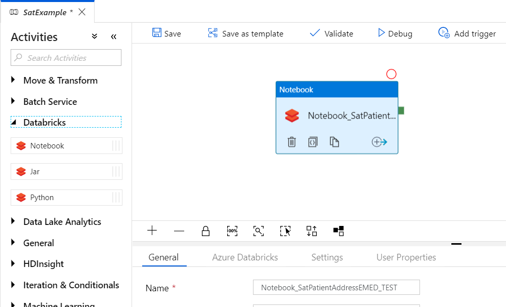Figure 2. Azure Data Factory Notebook Activity

On the Azure Databricks tab, select the Databricks cluster you created. Next, on the Settings tab we enter the path to our notebook and the parameter values we want to pass to the notebook:

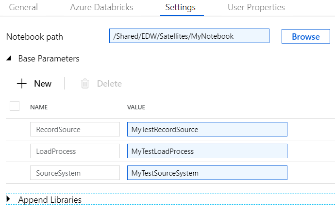Figure 3. Azure Data Factory Notebook Activity Settings Tab

And...thats it! You are now ready to run spark ETL pipelines in your Azure instance!

Loading JSON Files with Nested Arrays from Azure Blob Storage into Hive Tables in HDInsight

     In my previous post I wrote about how to upload JSON files into Azure blob storage. In this post, I'd like to expand upon that and show how to load these files into Hive in Azure HDInsight.

     
     The 2 JSON files I'm going to load are up in my blob storage, acronym/abc.txt and acronym/def.txt:

Figure 1. JSON Files in Azure Blob Storage

 Both of these files came from a public RESTful API:

http://www.nactem.ac.uk/software/acromine/dictionary.py?sf=abc

and

http://www.nactem.ac.uk/software/acromine/dictionary.py?sf=def


The format for these 2 files looks something like this:

{  
   "a":[  
      {  
         "sf":"ABC",
         "lfs":[  
            {  
               "lf":"ATP-binding cassette",
               "freq":1437,
               "since":1990,
               "vars":[  
                  {  
                     "lf":"ATP-binding cassette",
                     "freq":1057,
                     "since":1990
                  }
               ]
            }
         ]
      }
   ]
}

     First thing I'd like to do is create an external table in Hive, where I'm going to "load" the raw JSON files, so we can play around a little with some of the out of box Hive functions for JSON. In the Hive Query Editor 

DROP TABLE IF EXISTS AcronymRaw;

CREATE EXTERNAL TABLE AcronymRaw(json string)

STORED AS TEXTFILE LOCATION 'wasb://jymbo@jymbo.blob.core.windows.net/acronym/';

If we execute the following we can see the raw JSON:

SET hive.execution.engine=tez;

SELECT * FROM  AcronymRaw;

We will get back the raw JSON from the files. (I have to add the tez switch since I did not configure my cluster to use this engine by default). If I want to dive into the first array of my JSON objects and see the acronyms I can use a lateral view, to flatten out the hierarchy, combined with a  json_tuple function:

SET hive.execution.engine=tez;

SELECT

  b.sf

 FROM AcronymRaw AS a lateral view json_tuple(get_json_object(a.json, '$.a[0]'),'sf') b AS sf

Will give me:

Figure 2. JSON Acronym Results

If we want to step into the first array of the next level in the hierarchy, lfs, we can add another lateral view to the statement:

SET hive.execution.engine=tez;

SET hive.cli.print.header=true;

SELECT

  b.sf,

  c.lf,

  c.freq,

  c.since

 FROM AcronymRaw as a lateral view json_tuple(get_json_object(a.json, '$.a[0]'), 'sf', 'lfs') b AS sf, lfs

lateral view json_tuple(get_json_object(concat('{"a":', b.lfs, '}'), '$.a[0]'), 'lf', 'freq', 'since') c AS lf, freq, since;

Figure 3. First Nested JSON Array



     Now to get this JSON loaded into an external table, that will match the structure of the JSON, we're going to incorporate a 3rd party java library that can deserialize the JSON for us. This will make querying the data much easier. You can download and build the project using Maven from this github link, or you can be lazy, like me, and get the JARS from here. Using Visual Studio you can upload these files to blob storage so they can be referenced in Hive:

Figure 4. Visual Studio Server Explorer

       
     After adding these files to Blob storage we can reference them in our Hive statements when creating and referencing tables using this library:

ADD JAR wasb://jymbo@jymbo.blob.core.windows.net/user/hdp/share/lib/hive/json-serde-1.1.9.3-SNAPSHOT-jar-with-dependencies.jar;

ADD JAR wasb://jymbo@jymbo.blob.core.windows.net/user/hdp/share/lib/hive/json-serde-1.1.9.3-SNAPSHOT.jar;

DROP TABLE IF EXISTS AcronymNonNormalized;

CREATE EXTERNAL TABLE AcronymNonNormalized (

  a array<

    struct<sf:string,lfs:array<

          struct<lf:string, freq:int, since:int, vars:array<

                struct<lf:string, freq:int, since:int>

                  >

                >

              >

            >

          >

)

ROW FORMAT SERDE 'org.openx.data.jsonserde.JsonSerDe'

STORED AS TEXTFILE LOCATION 'wasb://jymbo@jymbo.blob.core.windows.net/acronym/';

     Now that this structure is in a Hive table, we can query it much easier than in the raw JSON format. In this query we can explode the lfs arrays and project them alongside sf:

ADD JAR wasb://jymbo@jymbo.blob.core.windows.net/user/hdp/share/lib/hive/json-serde-1.1.9.3-SNAPSHOT-jar-with-dependencies.jar;

ADD JAR wasb://jymbo@jymbo.blob.core.windows.net/user/hdp/share/lib/hive/json-serde-1.1.9.3-SNAPSHOT.jar;

SET hive.execution.engine=tez;

SET hive.cli.print.header=true;

SELECT

 

    a[0].sf,

    lfs.lf,

    lfs.freq,

    lfs.since

 

FROM AcronymNonNormalized LATERAL VIEW EXPLODE( a[0].lfs) lfstable AS lfs;

Figure 5. Exploded Results

     We can even drill into the second tier array vars using another lateral view and explode:

ADD JAR wasb://jymbo@jymbo.blob.core.windows.net/user/hdp/share/lib/hive/json-serde-1.1.9.3-SNAPSHOT-jar-with-dependencies.jar;

ADD JAR wasb://jymbo@jymbo.blob.core.windows.net/user/hdp/share/lib/hive/json-serde-1.1.9.3-SNAPSHOT.jar;

SET hive.execution.engine=tez;

SET hive.cli.print.header=true;

SELECT

 

    a[0].sf,

    lfs.lf as mainlf,

    vars.lf,

    vars.freq,

    vars.since

 

  FROM AcronymNonNormalized LATERAL VIEW EXPLODE( a[0].lfs) lfstable AS lfs

  LATERAL VIEW EXPLODE(lfstable.lfs.vars) vartable AS vars;

Figure 6. Second Nested Array

     
     So now that we've figured out how to traverse the arrays in the table, we could potentially normalize this table and create a schema similar to this:

Figure 7. Normalized Schema

 The first table we need to populate will be AcronymSF:

   ADD JAR wasb://jymbo@jymbo.blob.core.windows.net/user/hdp/share/lib/hive/json-serde-1.1.9.3-SNAPSHOT-jar-with-dependencies.jar;

ADD JAR wasb://jymbo@jymbo.blob.core.windows.net/user/hdp/share/lib/hive/json-serde-1.1.9.3-SNAPSHOT.jar;

SET hive.execution.engine=tez;

SET hive.cli.print.header=true;

DROP TABLE IF EXISTS AcronymSF;

CREATE TABLE AcronymSF

(

     sf string -->pk

);

INSERT OVERWRITE TABLE AcronymSF

SELECT

    a[0].sf

FROM AcronymNonNormalized;

SELECT * FROM AcronymSF;

Figure 8. Acronym SF Contents

     For us to populate the rest of the tables, we will need to produce unique values for the arrays in these hierarchies that will be part of a composite primary key.   To do this we will take advantage of a Hive function called posexplode that will generate an auto integer for each array so we can uniquely identify them. The first table we want to create and populate like this will be the AcronymLFS table:

ADD JAR wasb://jymbo@jymbo.blob.core.windows.net/user/hdp/share/lib/hive/json-serde-1.1.9.3-SNAPSHOT-jar-with-dependencies.jar;

ADD JAR wasb://jymbo@jymbo.blob.core.windows.net/user/hdp/share/lib/hive/json-serde-1.1.9.3-SNAPSHOT.jar;

SET hive.execution.engine=tez;

SET hive.cli.print.header=true;

DROP TABLE IF EXISTS AcronymLFS;

CREATE TABLE AcronymLFS

(

     sf string, -->pk

     lfs int, -->pk

     lf string,

     freq int,

     since int

);

INSERT OVERWRITE TABLE AcronymLFS

SELECT

    a[0].sf,

    lfstable.seq AS lfs,

    lfs.lf,

    lfs.freq,

    lfs.since

FROM AcronymNonNormalized LATERAL VIEW POSEXPLODE( a[0].lfs) lfstable AS seq, lfs;

SELECT * FROM AcronymLFS;

Figure 9. AcronymLFS Contents

     

     To load the AcronymVARS table we need to use the same method we used for AcronymLFS, but one level down on the JSON hierarchy:

ADD JAR wasb://jymbo@jymbo.blob.core.windows.net/user/hdp/share/lib/hive/json-serde-1.1.9.3-SNAPSHOT-jar-with-dependencies.jar;

ADD JAR wasb://jymbo@jymbo.blob.core.windows.net/user/hdp/share/lib/hive/json-serde-1.1.9.3-SNAPSHOT.jar;

SET hive.execution.engine=tez;

SET hive.cli.print.header=true;

DROP TABLE IF EXISTS AcronymVARS;

CREATE TABLE AcronymVARS

(

     sf string, -->pk

     lfs int, -->pk

     vars int, -->pk

     lf string,

     freq int,

     since int

);

INSERT OVERWRITE TABLE AcronymVARS

SELECT

    a[0].sf,

    lfstable.seq as lfs,

    vartable.seq as vars,

    vars.lf,

    vars.freq,

    vars.since

FROM AcronymNonNormalized LATERAL VIEW POSEXPLODE( a[0].lfs) lfstable AS seq, lfs;

LATERAL VIEW POSEXPLODE(lfstable.lfs.vars) vartable AS seq, vars;

SELECT * FROM AcronymVARS;

Figure 10. AcronymVARS Content

     So with this we have normalized our JSON. If we execute a standard SQL query in Hive like this:

SET hive.execution.engine=tez;

SET hive.cli.print.header=true;

SELECT

 

     tsf.sf,

     tlfs.lf AS mainlf,

     tvars.lf,

     tvars.freq,

     tvars.since

      

FROM AcronymSF tsf

JOIN AcronymLFS tlfs ON tsf.sf=tlfs.sf

JOIN AcronymVARS tvars ON tlfs.sf=tvars.sf AND tlfs.lfs=tvars.lfs;

We get this:

Figure 11. SQL Join Result

     

     As you can see from these results, they match exactly the results from the query in figure 6. Now for performance purposes you would want to leave all this data in the same table(nested arrays and all). But if you wanted to set this data up to be moved to a relational database with sqoop, going through this technique may be useful.